Statistical emulation and machine learning are widely used to predict and understand the behavior of complex systems such as those found in engineering and physical sciences. Machine learning models (aka emulators) are trained on data from simulations, tests, or other records and then used to rapidly predict system responses. These predictive models can be used for all kinds of sampling intensive analytics such as calibration, sensitivity analysis, optimization, and uncertainty propagation.
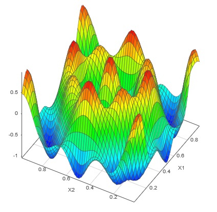
SmartUQ's breakthrough emulation algorithms dissolve barriers to fitting models to big data sets and high dimensional systems, opening new possibilities for the use of uncertainty quantification and analytics. Our patent-pending technologies easily handle continuous and discrete inputs, and can build lightweight emulators with univariate, multivariate, transient, and functional outputs. It does all this at lightning speed.
Emulators are statistical machine learning models that mimic the outputs of a complex physical or simulated system for a set of inputs. Building accurate high-speed emulators is a critical step in analytics and uncertainty quantification tasks. The dramatic increase in system evaluation speed and associated reduction in cost, going from a simulation or physical test to an emulator, allows you to perform many tasks that would otherwise be too slow or expensive. High-speed prediction of system outputs at any input configuration is invaluable for design space exploration, optimization, calibration, sensitivity analysis, and uncertainty propagation.
The larger and more complex the system, for example a jet engine simulation or test, the more advantage you will gain from emulation. While statistical emulators have shown promise in many challenges, they encounter serious numerical issues when applied to large scale or high-dimensional problems. Thus, building emulators with large and complicated data sets is widely considered a key bottleneck in analytics and uncertainty quantification.
SmartUQ has game changing emulation technology for larger data sets with many dimensions. Our accurate emulation techniques can quickly map out the entire input-to-output space of a complex system. We can fit a 1,000-point emulator in seconds and a 4,000-point emulator in minutes on a standard laptop. Using previous methods to build emulators for the same data sets can take hours or even days.
Example
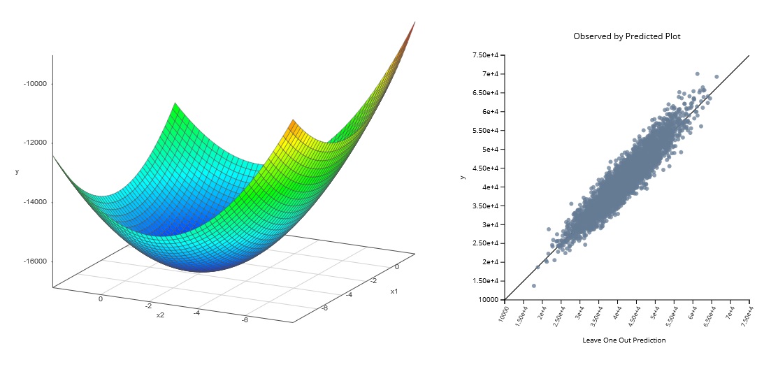 Large Scale Emulation
Multivariate response emulators are efficient for systems with a number of continuous inputs and multiple outputs such as automotive simulations and tests. Increased efficiency means users can explore and understand the relations between the different outputs and inputs simultaneously instead of individually, making the entire process faster than ever.
Example:
The emulator shown here was built to fit a 750-point data set with 10 input variables and 3 output variables. SmartUQ took less than 8 seconds to build this emulator on a typical laptop.
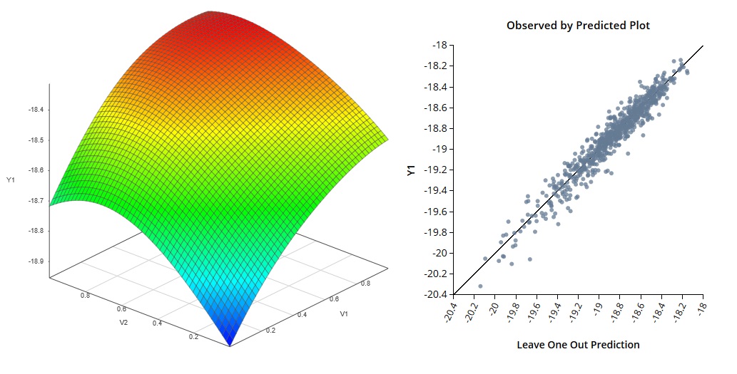 Multivariate Response Emulation Example 1
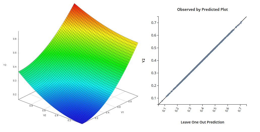 Multivariate Response Emulation Example 2
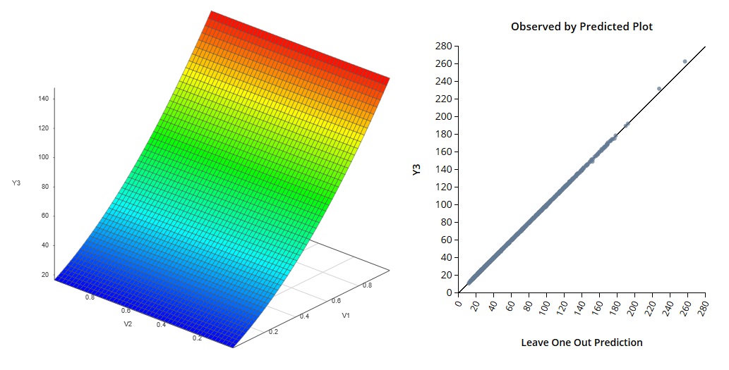 Multivariate Response Emulation Example 3
Mixed input emulators are useful when you handle systems with both continuous and discrete inputs. Discrete inputs can include things such as a set of fixed components, or even simulations including entirely different types of equipment or subsystem. Using mixed input emulation means you can build emulators for and analyze disparate designs with less effort. By considering more options at once you can create better designs.
Examples of discrete variables in an aircraft engine simulation might include using multiple different solvers, multiple discrete sizes and geometries of turbine blade, or multiple different types of turbine/compressor transmission.
One example of a mixed input problem is a radiation leakage model which might involve a continuous input, such as water flow rate, and a discrete input such as type of radioactive source material (e.g., contaminated equipment, fuel rods, glassified spent fuel).
Example:
This example was created using a univariate response mixed inputs emulator with six continuous inputs and one discrete input with five levels. SmartUQ took less than 9 seconds to build an emulator from the 500-point data set on a typical laptop.
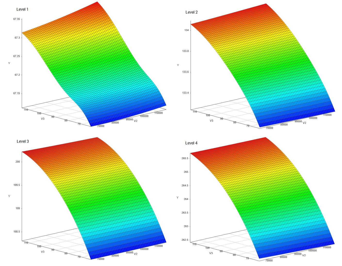 Mixed Inputs Emulation: Multiple Levels
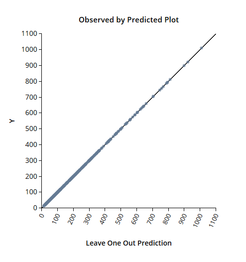 Mixed Inputs Emulation: Leave One Out Comparison
Simulations with functional or transient outputs are used scross all fields of engineering and physical science. Functional response emulators include at least one functional input variable, such as time or distance. For each simulation run, the outputs have values corresponding to the set of values of the functional inputs.
One example is an airfoil simulation which calculates surface drag. This simulation might have two functional input variables, time and distance along the length of the air foil, as well as a number of non-functional variables, such as average airspeed, surface coating type, and air foil cross-section geometric parameters. Each simulation is run with a set of the non-functional variables: e.g., only one surface coating type and geometry per simulation. The output, surface drag, is calculated at each time step and for each position along the length of the air foil and each simulation results in a function of the output variable with respect to the functional input variables. Thus, each input set of surface coatings and geometry configurations is associated with drag results over the length of the wing and for the time period of the simulation.
SmartUQ has a separate class of functional emulators to take advantage of the functional mapping of the input and output variables which makes emulator/surrogate model construction and use more efficient. There are usually orders of magnitude more functional input values, e.g. time steps or positions, than other input variables, which allows SmartUQ to emulate much larger functional data sets.
Example:
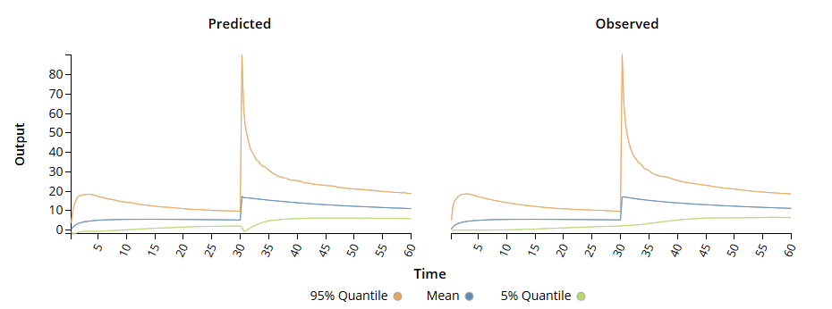 Transient Response Emulator Profile Comparison